When trying to find out if the UVP or method is suited to your application and will fulfill your measurement needs, several questions and criterias should be looked over:

• The medium of measurement should be a liquid.
• The presence of acoustic scatterers is a must and their characteristics should be such as their size is bigger than 10 microns and their acoustic impedance is not exactly equal to the one of the medium. See Scatterers.
• For velocity measurements, the velocity-depth range limitation has to be checked according to your measurement conditions: desired measurement depth and maximal velocity range. See Velocity.
• The depth vs medium attenuation, which is described here.
• If the spatial resolution is of importance, you should check the maximal reachable spatial resolution of our devices (see Technical specifications in the Products sections).
• If the time resolution is of importance, you should check the maximal reachable time resolution of our devices (see Technical specifications in the Products sections).
• For velocity measurements: the number of velocity components needed is also of importance. Several measurement techniques are described in the Technology section for 1, 2 or 3 components measurements, in average or instantaneous, depending on the needs.

If all those questions are answered and show the potential applicability of the UVP or ADVP measurement method, you can send your answers to us, so we can discuss with you which product is the best suited for your application. We could also schedule a demonstration on your setup, or a sample testing in our lab, to validate the feasibility and quality satisfaction.

If you want to perform accurate velocity or turbidity profile measurements on laboratory setup or industrial pipes, the UB-Lab is designed for you. Because it can control a wide variety of external transducers, it fits many purposes: flow visualisation in opaque liquids, flow metering in complex geometry, food quality control, concentration measurement, etc.

If you want to study and to monitor open channel, sewer flows or rivers, the UB-Flow is made for you. With its hydrodynamic and compact design, the UB-Flow is a fully integrated probe adapted to harsh environments. If the channel it too small, we will recommend to use the UB-Lab.

The UB-Flow is meant to measure in mainly horizontal flows. The most simple installation is to put the UB-Flow in the bottom of the flume. The UB-Flow has to be oriented in the main flow axis, the transducer "listening" towards the water surface and the head of the UB-Flow (side with the transducers) towards upstream.

It is also possible to attach the UB-Flow on a flume wall for example (side looking), measuring then horizontally.

Installation on a floating board is also possible for down-looking setup.

Yes, but the material of the wall is of great importance. To optimise the propagation of ultrasounds, the material should not contain particles nor fibers and in particular its acoustic impedance should approach the one from the liquid in which you want to measure. The greater the difference, the less the ultrasound will be able to penetrate into the liquid. It is very easy and common to measure through plastic walls for example.

Also, as high frequency ultrasounds does not penetrate air properly, any air layer or big bubble across the acoustic beam should be eliminated. This is why, when measuring through a plastic wall for example, the user has to put ultrasonic transmission gel between the transducer surface and the wall, making sure the gel layer does not contain bubbles. And when measuring through a wall, it is recommended to activate the static echo filter.

Our transducers can be immersed in water. Standard transducers resist at temperatures between 0 and 40°C, and a pressure up to 4 bars. Our HT transducers resist at temperatures up to 110°C.

If you are using other liquids than water, you should check with us if they are compatible.

No, at the emission frequencies we work with (0.8 to 10MHz), the ultrasound does not penetrate air properly to do measurements.

For detailed informations about the influence of a particle’s characteristics on the recorded RMS (root-mean-squared) voltage of the backscattered signal, you can have a look on this article and this thesis:

• Schmitt (2016): Suspended Sediment characterization by Multifrequency Acoustic, Philippe Schmitt, Anne Pallarès,Stéphane Fischer and Marcus Vinicius de Assis, 2016, ISUD10.
• Bricault (2006): Retrodiffusion acoustique par une suspension en milieu turbulent: application à la mesure de profils de concentration pour l'étude de processus hydrosédimentaires, Mickaël BRICAULT, 2006, INP Grenoble.

Usually, the natural particle contamination of water is sufficient for UVP Monitor measurement. But if the medium is too clean or if you want to improve your measurements, you can introduce tracing particles in you flow. These particles can be from a little bit mud in hydraulic models for example. But there are also artificial particles you can use: glass spheres or polyamide particles. If you are lost, you can have a look on the particles selected by Ubertone.

Basically, when you choose your particles, you will be able to choose their size, density and shape. And usually, you want to have influence on the size, on the sedimentation velocity and on the acoustic impedance of the particles.

The particles should have a low Stokes number to follow the flow, ...

Stokes’ formula gives:

where µ is the dynamic viscosity of the medium, r is the particle radius, g the acceleration of gravity and

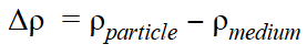
the mass density difference between the particle and the medium.
Small size and a mass density as close to the medium’s as it is possible lead to a small sedimentation velocity.

... they should have an acoustic impedance that allows to have a good amplitude of signal ...

Le acoustic impedance of a matter is given by

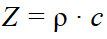
where c is the sound velocity in this matter and the mass density of the same matter. The amplitude of the signal scattered by the particle depends on Zpthe acoustic impedance of the particle matter and on Zmthe one of the medium:

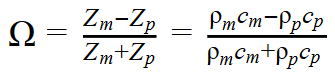
and if the medium is water,

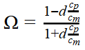
where d is the particle matter density.
This means it is actually the difference of mass density and of sound speed between the medium and the particle that leads to more signal.

… and they should be big enough to be seen by the ultrasounds.

We know that the particles should be equal or smaller than the wavelength of the ultrasound wave. But if they are too small, they won’t scatter enough to be seen by the transducer. There is no magical formula to calculate the minimal size given the wavelength. Arbitrarily and given our experience, we could say that 2% of the wavelength should be a good limit.

Ubertone has selected and characterised polyamide particles which fit perfectly to our devices and transducers. For more information, you can have a look at the particles product page.

When measuring the velocity by coherent Doppler method, the visibility may be limited by the presence of ghost echoes (or phantom echoes), i.e. echoes from a previous pulse. In this case, it is possible to filter them by using pulse coding method which is part of a unique technological system devised by Ubertone.

Any monostatic system (the same transducer is used as emitter and receiver) presents a blind zone, just in front of the transducer. In this area, the signal-to-noise ratio is low due to the prior ultrasonic emission. The length of this area depends on the transducer design, the emitted frequency and the concentration of particles. Thanks to Ubertone’s transducer design and specific signal processing of our hardware, the length of the blind zone is very short, typically within 2 to 20 mm.

If there are bubbles and microbubbles in your setup, and in particular when your transducers are oriented downwards, small bubbles will get attached to the transducers active surface.

As this measurement technique does not work through air, when too many bubbles clog up the transducers, the data quality will be affected and may become very poor. You will witness this especially by observing the Doppler Signal-to-noise ratio (SNR).

There are several leads that can help you go around this issue:

• The most efficient is to get the whole transducers holder out of the water and plunge it in again.

  If you have a motorized carriage for example, this can be done automatically. And if you wish, you can connect your carriage to the trigger inputs of the UB-Labs not record the moments out of water.

• The other more simple version is to wipe the transducer surfaces manually.

• In some cases, the flow is strong enough to flush the bubbles away. One idea, which we have not tried out yet, would be to have a system of water jet ejection near the transducer surface, but the absence of influence on the zone of interest should be checked.

Hereby we would like to explain the importance of using a second transducer when measuring flow velocities with the monostatic technique.

Indeed, using only one transducer should only be applied for qualitative measurements or in the case of pipes with a long enough strait section to make the assumption of a well known flow direction.

But in most cases, such assumptions will lead to errors of interpretation, and there are secondary currents.

Concerning the influence of the error on the angle with a single transducer:

$${{\Delta U} \over {U}} = tan(\beta)⋅\Delta \beta$$

In the case of 75° with 1° error on the transducer angle, the error on the velocity is 6.5%. And if you consider that there is a small secondary current, for example \(w = 0.05⋅u\), then the error on the u velocity may reach 25% !

With two transducers, the combination is done as shown here, and the error can be expressed as:

\({{\Delta U} \over {U}}={{\Delta \epsilon} \over {sin(\epsilon)}}\) with \({\epsilon}={\beta_2 - \beta_1}\)

In the case of 75° and 105° with 1° error between the two transducers, the error on the velocity is 3.5%.

If the holder is 3D-printed or machined, it is much easier to get a good accuracy on the angle between the transducers than for a single transducer in a given setup. And, most importantly, there will be no influence of secondary currents, plus the average w-component will also be measured.

In conclusion, when using a single transducer, the positioning error has a strong impact and, in addition, any small secondary current will strongly affect the error on the measured velocity. On the other hand, when using two transducers in a holder, the error due to the uncertainty on the transducer’s angle is lower and the secondary currents have no influence on the velocity measurement.

I can make a UB-SediFlow out of my UB-Lab

...read more

If you are using a UVP (UB-Lab UVP or UB-Flow) for the first time, you can follow the tips below.

The most simple way to set a UVP up when you start using it is to use our web interface. You can activate the "help" option by going to the "preferences" page.

• The emission frequency can be set to the central frequency of the used transducer.
• Then, you have to adjust the PRF (pulse repetition frequency) which depends on the velocity range you wish to measure (see How to know the maximal measurable velocity for my setup? What is the Range-velocity ambiguity?).
• Set the minimal measurable velocity. You will then see in the "information" box in the top right corner the maximal measurable velocity it allows you to measure.
• Concerning the profile dimensions (position of the first volume, inter-volume distance and number of volumes), it depends on your setup. Set the volume size equal to the inter-volume distance is often the best and simplest way to begin. You will see the maximal depth over which you could measure, imposed by the PRF, and the depth over which you will effectively measure.
• Next, you set the number of pulses to the maximum; this is the number of pulses used to measure an instantaneous profile. And you decide the number of instantaneous profiles over which you want to do the average. This will lead to an instantaneous measurement time and to an average (bloc) measurement time indicated in the same "information" box.
• At last, for the first measurement, il is better to activate the pulse coding, the static echo filter and the automatic gain control.

You are ready to measure!!

WARNING: To measure acoustic turbidity, the setup is different.

The velocity measurement by coherent pulsed Doppler technique gives an excellent spatial and temporal resolution combined with a very good accuracy, thus in a given limit of velocity range.

The repetition of the ultrasonic pulses gives a precise measurement of the Doppler phase in a small cell (or volume of fluid). Nevertheless, this approach induces a limitation of the velocity range for a given exploration depth. Thus, the pulse repetition period defines on one hand the exploration depth (all the echoes will have to come back from the medium before the next pulse is sent) and on the other hand the interval for the determination of the Doppler shift (between -π et +π and proportional to the velocity). When the interval between two successive pulses is too long, the measurement suffers from a phase jump inducing an ambiguity. On a frequency point of view, this is equivalent to overstep the limit given by the Nyquist-Shannon theorem.

This phase jump results in a velocity jump that can be observed on a profile with a velocity gradient. The figure above shows the measurement on a profile with velocity increasing with the depth. The red lines shows the velocity limits of the range; one can see that each velocity outside this range suffers from a jump that brings it inside the interval.

Thus the instantaneous velocities (in green) are reduced in negative values when they overstep the highest limit of the range.

The velocity range for the projected velocities (as measured by the device) is given by:

with: PRF the Pulse Repetition Frequency, c the sound speed (about 1480m/s in water), f₀ the emitting frequency.

Finally, it is the pulse repetition frequency (PRF), defined in the setup, that will act on one side on the maximal exploration depth and on the other side on the maximal velocity. This limit is expressed by:

with : R_v the velocity range along the flow axis, R_y the exploration depth (orthogonal to the main flow direction, the pipe diameter for example), β the angle between the beam axis and the velocity vector. In monostatic mode, the velocities measured are those projected on the beam axis of the transducer used to measure. This is why, because of the geometrical uncertainty and mainly because of the turbulences, the angle between the beam axis and the velocity vector can not be too near to 90°.

Pulse coding is a unique technique implemented in Ubertone’s profilers that removes the effect of parasitic noises on the velocity profiles.

These parasitic noises may be of several kinds:

• ultrasonic noise generated by external sources (pumps, waterfall, pipe vibrations, etc.),
• electromagnetic noise generated by external sources (electrical engines, variable speed systems using a frequency inverter, etc.),
• ghost echoes from the previous acoustic pulses generated by the profiler itself.

Ghost echoes (also known as phantom echoes in ultrasonic testing) come from intense scattering area or reflection on walls or objects. They particularly occur when working:

• at low emitting frequencies,
• in closed tanks,
• in small pipes and channels with rough surface,
• at a high PRF (pulse repetition frequency).

When any of these noises has a frequency signature (and it is usually the case), a standard profiler will interpret this as a Doppler shift and will cause an important bias in the velocity profile. This is shown by the red profile on the graph below where a ghost echo introduces an error in the velocity measured in a closed pipe. When the pulse coding is activated, these noises are not taken into account by the signal processing of Ubertone’s profilers so that the estimated velocity corresponds accurately to the velocity of the flow at the given position (green profile in the graph).

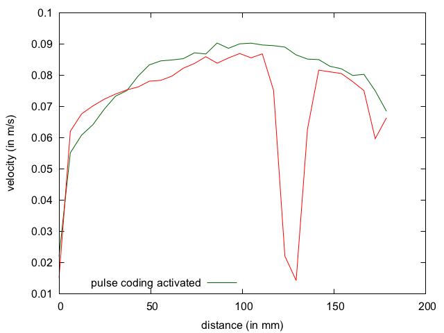
This technique is part of the intellectual property of Ubertone. Each emitted pulse is coded. This allows the receiving electronic to distinguish the signal coming from the last emitted pulse from any other parasitic noise. If the energy of the parasitic noise is too strong compared to the energy of the signal, the standard deviation of the velocity measurement will be affected. In this case, the affected velocity points can easily be removed by using a threshold on the SNR (Signal-to-Noise Ratio).

When a cell (i.e. single measurement volume) contains both a static wall (or any motionless object) and moving particles, the estimated velocity will be the average between the wall velocity (which is zero) and the particle velocities (considered equal to the liquid flow velocity). This average is weighted by the energy of the respective echoes. As the echo of a wall may be much stronger as the echoes from scattering particles, the wall will introduce an important bias in the velocity estimation.

The static echo filter implemented in Ubertone’s devices is a numerical processing that removes the effect of motionless objects in order to get only the velocity of the moving particles.

This filter is very useful when measuring through a wall.

Ubertone’s devices are equipped with an automatic gain control algorithm that optimizes the gain over the full observed window with a logarithmic law. It is thus recommended to limit the number of cells to the area of interest so that the gain is well adapted to this area (and not influenced by the echoes after an interface for example).

The transducer emits a pulse (short burst) of a specified duration into the liquid. This ultrasonic pulse consists of several periods at the carrier frequency (emission frequency) within the bandwidth of the transducer. By traveling into the liquid, the pulse will form an acoustic beam.

This acoustic beam (for a round transducer) is firstly contained in a cylindrical shape in said near field, in which the energy has a complex distribution. This cylinder has a diameter D defined by the active part of the transducer. The beam then takes a conical form in the region of the far field, where the distribution of the acoustic energy is more uniform. The limit between the two regions is defined by the near field distance (rnf) that is set at the largest peak furthest from the transducer:

$$r_{nf} = {{D^2⋅f_0} \over {4⋅c}}$$

The geometric transition between the cylindrical and conical shape of the beam takes place at about 1.6 times the near field distance.

$$\alpha = {{1.22⋅c} \over {D⋅f_0}}$$

An acoustic configuration is the set of parameters that the instrument needs to know to do a measurement. In our profilers, those parameters are for example: the emission frequency, the number of cells in the profile, the cell size, the pulse repetition frequency, the number of samples to estimate one velocity, etc. Our instruments can memorize several acoustic configurations that are executed sequentially during the recording. The record unit is a block of several profiles obtained following one configuration. One record cycle consists in measuring one block of each configuration.

For more details, you can ask for the user manual.

One record consists of a series of record cycles. One record cycle consists in measuring one block of each configuration. Each block results in an arithmetic average of n_profile measured profiles (velocity, SNR and echo amplitude). The delay required to obtain one averaged profile is approximately equal to:

$${{n_{ech} ⋅ n_{profile} } \over {PRF}}$$

\(n_{ech}\), the number of samples for one instantaneous velocity estimation and \(PRF\) the pulse repetition frequency.

Thus the duration of a record cycle is at least equal to the sum of the Average measurement duration of each configuration.

Due to the hardware’s architecture, there is a delay between each block. Thus the duration of one record cycle is at least equal to the sum of the average measurement duration of each configuration plus the inter-block delays.

Inside of one block, the single (instantaneous) measurements happen one after the other in an optimised manner, allowing to reach high sampling frequencies.

• For the UB-Lab X2, X8 (and 2C manufactured before 2023), the inter-block delay is 0.5 to 1s. Thus the technical specification of "up to 100Hz" refers then to the sampling frequency of instantaneous profiles at \({n_{ech} \over {PRF}}\) within one block. Those instantaneous profiles are stored in a raw binary data file for space optimization.

  The number of profiles per block has to be at least 1. And we added a limitation on the maximum number of profiles per block to avoid data overflow. But there is still a risk of overflow during a block as we run on an embedded OS.

  Thus, it is advised to close the graphical interface during the record.

  This limitation is based on the number of cells per second (CPS) that the system is able to manage.

  For each processed configuration, the system tries to acquire a complete bloc. If it fails to get a complete bloc, the system switches to the next bloc (if only one configuration) or to the next configuration. For more details, you can ask for the user manual.

  \(n_{ech}\)	\(n_{vol}\)	\({PRF}\) (Hz)	Sampling rate within a block (Hz)	Maximum guaranteed \(n_{profile}\)	Potential maximum \(n_{profile}\)
  64	50	1000	16	130	7196
  64	50	3000	47	130	3452
  64	100	1000	16	65	5128
  64	100	3000	47	65	771

• The UB-Lab P, S4 and UB-SediFlow do not provide the instantaneous measurements, but only the block averaged profiles. In this case, technical specification refers to the sampling frequency of the blocks.

Summary:

	UB-Lab X2, X8, (and 2C manufactured before 2023)	UB-Lab P, S4 and UB-SediFlow
Sampling frequency	up to 100Hz (of instantaneous profiles within one block)	up to 15Hz (of the blocks)
Transducer channel switching delay or delay between blocks	500 to 1000 ms	10 to 200ms (typical)
Data overflow risk	see example above	no limitation

• When activating the trigger option on the UB-Lab X2/X8/2C and starting a record, the device will do one unique block measurement when it detects a trigger rising edge. If there are several configurations set, it will switch to the next configuration and do a block measurement with this one at the next trigger rising edge. The delay between rising of trigger and first pulse depends on the configuration, and ranges between 46 and 1000μs, but this delay is constant for one configuration during the recording.
• For the UB-Lab P, the trigger input signal enables the storage of data. During a recording session, the device measures continuously, but only blocks where the "trigger" signal is at high level (at the beginning and the end of the block) are effectively stored in the record file. The delay between rising of trigger and taking into account is up to 5ms plus the block duration.

Summary:

		UB-Lab X2, X8, 2C	UB-Lab P
\({Td}_{out}\)	Delay between rising of trigger and first burst and between the last burst and the falling of trigger	45 to 160µs with jitter=120µs	1 to 5ms
\({Td}_{in}\)	Delay between modification of trigger and taking into account (with 𝛕 : block duration)	/	1 to 5ms+𝛕
	Delay between rising of trigger and first pulse (depend of the configuration)*	46 to 1000µs	/

* This delay is constant for one configuration during the recording

The PRF (Pulse Repetition Frequency) is a very important parameter in the pulsed coherent UVP and ADVP measurement technique.

It is the frequency at which the pulse trains (or bursts) are sent into the medium.

It defines the time resolution of the measurements. The higher the PRF, the higher the sampling rate (see FAQ - What does the announced sampling rate exactly refer to?).

And it defines the measurable velocity range, and the maximal available depth:

• For the velocity range, see FAQ - How to know the maximal measurable velocity for my setup? What is the Range-velocity ambiguity? (also called ambiguity). The higher the PRF, the wider the velocity range, thus potentially the higher the maximal measurable velocity.
• On the other side the lower the PRF, the higher the maximal available depth.

In most cases, the higher the PRF the better.

Nevertheless, following elements need to be taken into consideration:

• the higher the PRF, the higher the risk of parasitic and ghost echoes (see FAQ - What are ghost echoes?). These parasitic echoes will appear even more and stronger compared to your signal of interest when working with low concentrations and small/closed setups. Thus it may be of interest to compare regularly the backscattered echo amplitude profile measured at high PRF with a short measurement at low PRF to check that there are not too many parasitic echoes.
• the higher the PRF, the bigger the velocity resolution. Thus a high PRF is not well suited to measure low velocities. It is better to adapt the PRF to the effective velocity range as much as possible.

See also: FAQ - How to setup a UVP for velocity measurements?

The raw velocity, ie. the projected velocity on the transducer axis, is given by:

$$ v_p = {{c⋅f_D} \over {2⋅f_0}} $$

The velocity accuracy given in the technical specifications of our UVPs is the accuray on the velocity projected on the transducer axis. It is based on the accuracy of the electronic components which determines the Doppler frequency fD.

The sound speed needs to be well known. In fresh water, it only depends on the temperature.

As an indication, here is the application of the relative error of sound speed for a temperature of (25±1)° C : $$ {{\delta c} \over c} = {2.67 \over 1496} = 0.18 \% $$

When projecting the raw velocity on any other axis, the uncertainty on the angle of installation of the transducer has a great influence. See FAQ - What is the interest of using two transducers for monostatique measurements?

The velocity resolution given in the technical specifications of the UVPs is the resolution of the velocity projected on the transducer axis.

It is given in ppm (parts per million) of the velocity range. Indeed, the velocity resolution depends on the set measurement parameters defining the velocity range, see UVP velocity measurement principle

Thus, when setting the PRF (Pulse Repetition Frequency), make sure the velocity range is not excessively large compared to the effective velocities in your setup.

The velocity resolution of Ubertone’s UVPs is the best available on the market.

The turbidity (the cloudiness of water) is due to the presence of suspended matter or sediments composed by organic and inorganic particles, flocs or vesicles.

For more details, see Acoustic turbidity measurement.

This is part of Ubertone’s philosophy : a scientific instrument shall measure data without any assumption on the medium in order to provide reliable information.

Thus, we choose to separate clearly measurement from specific processing. On one side we provide instruments that measure profiles (velocity, SNR, echo and acoustic turbidity). On the other side we provide a set of processing tools (cloud2.ubertone.eu) that allow the user to visualize, analyse and post-process their data.

Multi-component velocity measurement along a profile allows the observation of the orientation of the flow as a function of depth.

UBERTONE’s profilers allow the access to this data through:

• a monostatic combined multi-beam technique (2C or 3C) UVPs. For example with the UB-Lab X8, it is possible to combine multi-beams for average localised 3C or to mimic a divergent 4-beam ADCP with a high spatial resolution (over the beam axis) but limited to about 0.1Hz. The UB-Flow, embedding two transducers for field applications, can provide 2C average velocity profiles by post processing.
• or a bistatic measurement technique with: our UB-Lab 3C allowing high spatial and time resolution 2C and average 3C profile measuring.

As a lot of options are available, our profilers prices depend on which measurement technique and specifications you need, depending on your application or setup. The price of our standard profilers (from a UVP UB-Lab (UVP) starter kit to a 3C ADVP, the UB-Lab 3C) can vary between 17500 and 72000€.

For custom designs, feel free to contact us.

The price of our OEM profilers depends on volume.

For more information, you can have a look at our How to purchase ? page.

No, the UB-Flow is not a flowmeter. But as it can measure velocity profiles and as the water height can be calculated from the measured echo amplitude profile, if the section is well known, the user can calculate a flow rate from the measured data. The UB-Flow has been designed for research applications.

By the way, UB-Analytics, UBERTONE’s cloud and post-processing tool, provides a function to detect the water level.

Nevertheless, the UB-Flow AV is an average flow velocity monitoring sensor. It aims to equip flowmeters for sewer networks monitoring.

For more information, feel free to contact us.

There are three major advantages of acoustic instruments over optical ones, the first being the ability to measure in opaque liquids. As soon as there are scatterers in the liquid, the acoustic instrument will detect them and be able to get their velocity.

This argument goes hand in hand with the ability to measure through opaque walls. Optical instruments are even sensitive to dirty walls, which lead to a weak signal.

The second advantage is the easy installation. UVPs for example need only one transducer installation to get first measurement data. Also, Ubertone’s GUIs are web based and embedded in the devices, requiring no software installation and allowing to use the device directly after unpacking. The UB-Lab P even allows a wifi connection with your smartphone.

The third advantage is the cost: see FAQ How much does a profiler cost ?.

You may be lost in all these acronyms ! Here are some explanations and historical facts. Even if they are all related to velocity measurement by use of acoustic techniques, they correspond to different emission/reception and signal processing techniques.

The UVP (Ultrasonic Velocity Profiler) technique has been introduced to Fluid Mechanics by Takeda (1986). It is also known as UDV for Ultrasonic Doppler Velocimetry and was originally applied in the medical field. This technique based on coherent Doppler allows to measure velocity profiles with a high spatial and temporal resolution. Since then, many researchers have shown promising applications, especially in flow metering, rheometry, flow mapping and environmental flow studies. On the other side, the ADCP (Acoustic Doppler Current Profiler) technique (firstly derived from oceanographic sonars) is dedicated to long range measurement using pairs of long coded pulses inducing a low spatial resolution with a large velocity range. But ADCP devices are designed to fit for outdoor applications.

Both UVP and ADCP use the monostatic method, getting one velocity component per measurement and per beam. Thus, only averaging over time and space allows to get multi-component velocity profiles, by making (strong) assumptions and by combining several measurements on several measurement lines (transducers). In a certain way, UVP (or UDV) can be considered as a high resolution ADCP.

The multi-bistatic technique provides an instantaneous two or three components (2C/3C) velocity measurement. The ADV (Acoustic Doppler Velocimeter) includes one emitter and 3 or 4 receivers receiving at the same time and gives the instantaneous 3C velocity in one single volume in front of those transducers.

The ADVP (Acoustic Doppler Velocity Profiler) was designed at the EPFL in Switzerland (Rolland et al. 1997), it refers to an ADV with a profiling capability. It includes one emitter and at least 2 receivers receiving at the same time, but the received signal is sampled along time to get instantaneous 2C velocities over a measurement line resulting in an instantaneous 2C velocity profile measurement. The addition of simultaneous receivers allows the obtention of the third component.

The ACVP (Acoustic Concentration and Velocity Profiler) was designed at the LEGI in France (Hurther et al. 2011) and is an ADVP with post-processing of the acoustic echo amplitude signal to get the particles concentration along the same line as the velocity profile.

Ubertone offers acoustic velocity profiler for laboratory and field studies:

• several UVP/UDV solutions:
  • the UB-Lab P, X2 and X8 for laboratory applications,
  • the UB-Flow for outdoor applications,
  • and the Peacock UVP for OEM embedding.
• an ADVP solution: the UB-Lab 3C.

Takeda Y. (1986). Velocity profile measurement by ultrasound Doppler shift method, International Journal of Heat and Fluid Flow, 7(4), December 1986, 313-318.

Rolland, T.; Lemmin, U. (1997). A two-component acoustic velocity profiler for use in turbulent open-channel flow. Journal of Hydraulic Research, 35(4), 545–562.

Hurther, D., Thorne, P.D. Bricault, M., Lemmin, U., Barnoud, J.-M. (2011). A multi-frequency Acoustic Concentration and Velocity Profiler (ACVP) for boundary layer measurements of fine-scale flow and sediment transport processes. Coast. Eng., 58(7), pp.594–605.

We listed here a few differences between the UB-Lab P and the UB-Lab X2/X8, which will help you to choose the UVP that is best suited for your needs.

	UB-Lab P	UB-Lab X2/X8
communication	wifi : makes it more simple and robust to connect with the instrument	Ethernet
on/off	button	through GUI
Power supply	embedded battery : no risk to damage the system on power down	mains power supply
Emitting frequency	0.025 to 3.6MHz	0.8 to 9.4MHz
real-time visualisation	average and standard deviation velocity profiles, echo amplitude, SNR	instantaneous and average velocity profiles, echo amplitude, SNR
record and file management	manual start/stop	settable record duration and intervals
maximum acquisition rate on a single transducer	15 Hz continuously	100 Hz within small blocks separated by 0.5 to 1 second, see FAQ-Sampling rate
maximum acquisition rate when switching between different transducers	15 Hz	1 Hz
jitter between 2 profiles	4 ms	0.1 µs

In addition to a more advanced GUI in the UB-Lab P, what comes mainly out of this analysis is that the UB-Lab P fits most applications in a robust manner. The only reason to use the X2 or X8 is :

• when high acquisition rate is needed (on a single transducer only)
• when measuring at a high emitting frequency is required
• when more than 2 transducers need to be managed: UB-Lab X8

You can see the detailed specifications of those devices in the UB-Lab P family page

It is necessary to take good care of your cables. The transducer cables are especially important to take care of, as they are linked to the transducer head and need to maintain their waterproofness, shielding and link to the piezo (of course).

Learn more!