Ubertone

Ubertone’s profilers allow to make accurate velocity and echo amplitude profile measurements at high spatial and high time resolution.

Our technology is inspired from medical imaging and oceanographic sonar and also known as UVP (Ultrasonic Velocity Profiler) or UDV (Ultrasonic Doppler Velocimeter)

Measure with this technique requires :

a hardware for the emission and reception of ultrasonic pulses and signal processing, and
a probe, called transducer, for the transmission of acoustic pulses into the medium and the transmission back of the echoes as an electric signal to the hardware.

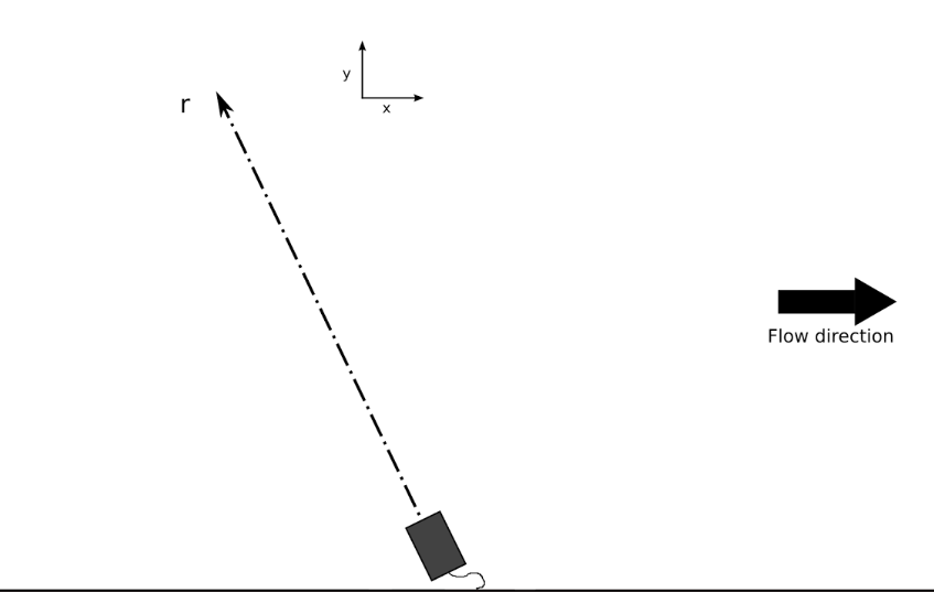
Geometrical conventions

Two different reference frames may be used: the transducer reference frame and the flow reference frame.

r : distance to the transducer over the beam axis (included in (x,y) plan),
x : main flow direction,
y : orthogonal to the main flow direction (axis in the flow section).

By convention, the velocity is positive whenever the liquid is flowing towards the transducer.

Measurement cell

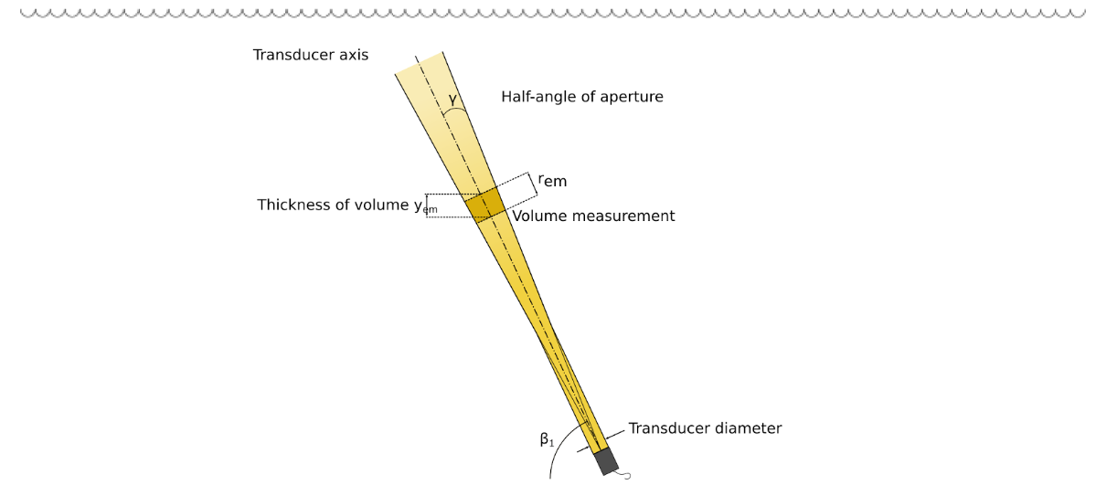
The transducer emits a burst of a specified duration into the liquid. This ultrasonic pulse consists in several periods at the emission frequency (carrier frequency) within the bandwidth of the selected transducer.

The acoustic beam starts with a cylindrical shape with same diameter as the transducer.

Then, after roughly 1.6 times the near field distance ($r_{nf}$), the beam turns into a conical shape (of half-angle spread $\alpha$) :

$$r_{nf} = {{D^2⋅f_0} \over {4⋅c}}$$

$$\alpha = {{1.22⋅c} \over {D⋅f_0}}$$

The measurement cell is defined as a slice of the beam with a thickness defined by emission pulse duration, thus defining the spatial resolution. The diameter of the cells changes along the depth and can be obtained from the diameter of the beam. The thickness of the cells is constant and given by:

$$r_{em} = {{c⋅n_{em}} \over {2⋅f_0}}$$

and: $$y_{em} = r_{em}⋅\sin{\beta}$$

with:

$r_{em}$: cell thickness [m] along the beam axis,
$c$: sound speed in the medium [m/s] (around 1480m/s in water),
$n_{em}$: number of periods at the carrier frequency inside the emitted burst,
$f_0$: emission frequency [Hz].

During the setup, the user defines the value of the projection of the thickness along the axis in the flow section, $y_{em}$.

The intensity of the acoustic beam decreases with the distance and thus induces a physical limit to the exploration depth. Indeed, while propagating, the ultrasonic waves concede a part of their energy to the medium by scattering and absorption.

Profile measurement

The measurement of a profile by the mean of an ultrasonic wave supposes the presence of acoustic scatterers in suspension in the fluid. The acoustic scatterers may be particles, micro-bubbles, vesicles or any local variation of the acoustic impedance.

After emitting the ultrasonic pulse, the system switches in receive mode. The acoustic wave propagates along the beam axis and each scatterer that crosses the beam will diffuse an echo toward the transducer. The echo of a given particle will reach the transducer after a time of flight (back and forth) equal to $2r \over c$, with :

$r$ : distance between the transducer and the scatterer [m],
$c$ : sound speed in the medium [m/s].

The scatterers dispersed in the flow will allow to obtain a continuous backscattered signal from the medium. This acoustic signal is composed, at a given time, by the sum of the echoes of the scatterers located, at a given distance, in the measurement cell.

The regular sampling and analysis of the backscattered echo allows to obtain a so called profile. A profile can be considered as a vector of a physical quantity distributed along an axis.

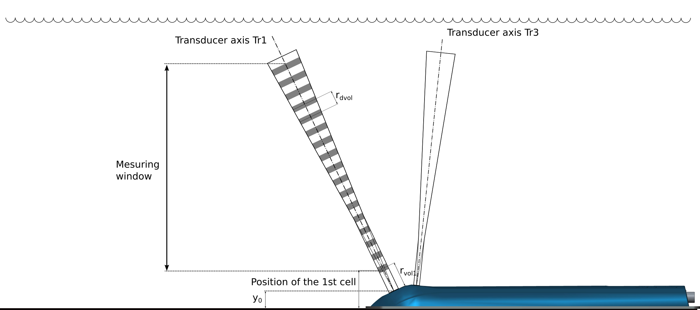
The attached illustration shows the measurement window, the position of the first measurement cell and the inter-cell distance. The position of each cell is defined by its centre.

The inter-cell distance is the distance between the centre of two successive cells.

As for the cell thickness, the user defines, in the software interface, the value of the projection of the inter-cell distance over the flow section axis (vertical).

One instantaneous profile is obtained by sending a series of $n_{ech}$ pulses and analysing the corresponding backscattered signal.

The pulses are sent at a frequency called $PRF$ (Pulse Repetition Frequency). The $PRF$ is chosen so that all the echoes from the medium have been received before sending the next pulse.

The time delay needed to obtain one instantaneous profile is equal to $n_{ech} \over PRF$. By choosing a high number of samples with a low $PRF$, the measurements may be slowed down.

Instantaneous profiles are sampled continuously inside one block. A block is composed of $n_{profile}$ instantaneous profiles. Thus, the time delay needed to obtain one averaged profile is equal to $n_{ech}n_{profile} \over PRF$.

Doppler Effect

The acoustic scatterers, moving with the liquid flow with a velocity $\overrightarrow{V}$, will induce a frequency shift in the backscattered signal: the Doppler shift.

In each cell, the information obtained from the $n_{ech}$ pulses is used by the instrument to estimate the projection of the velocity vector over the beam axis. The measured velocity can be expressed as:

$$V_p = {{c⋅f_D} \over {2⋅f_0}}$$

$V_p$: velocity projection [m/s],
$c$: sound speed in the medium [m/s],
$f_D$: Doppler frequency [Hz],
$f_0$: emission frequency [Hz].

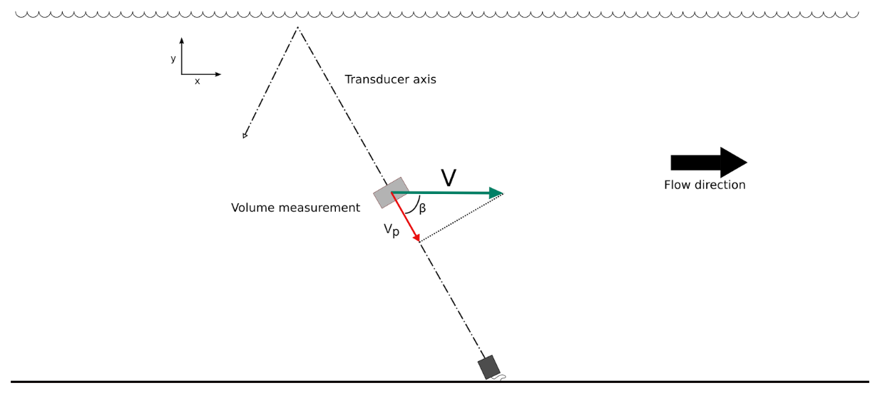
When the angle $\beta$ (between the measurement axis and the flow axis) is known, the flowing velocity $V$ (see Illustration) along the horizontal axis may be calculated from:

$$V = {V_p \over \cos{\beta}}$$

See this FAQ to understand why it is interesting to use a second transducer for monostatique measurements.

Range-Velocity Limit

The velocity measurement by coherent pulsed Doppler technique gives an excellent spatial resolution combined with a very good accuracy, thus in a given limit of velocity range.

The repetition of the ultrasonic pulses gives a precise measurement of the Doppler phase in a small cell. Nevertheless, this approach induces a limitation of the velocity range for a given exploration depth. Thus, the pulse repetition period defines on one hand the exploration depth (all the echoes will have to come back from the media before the next pulse is sent) and on the other hand the interval for the determination of the Doppler shift (between -π et +π and proportional to the velocity). When the interval between two successive pulses is too long, the measurement suffers from a phase jump inducing an ambiguity. On a frequency point of view, this is equivalent to overstep the limit given by the Nyquist-Shannon theorem.

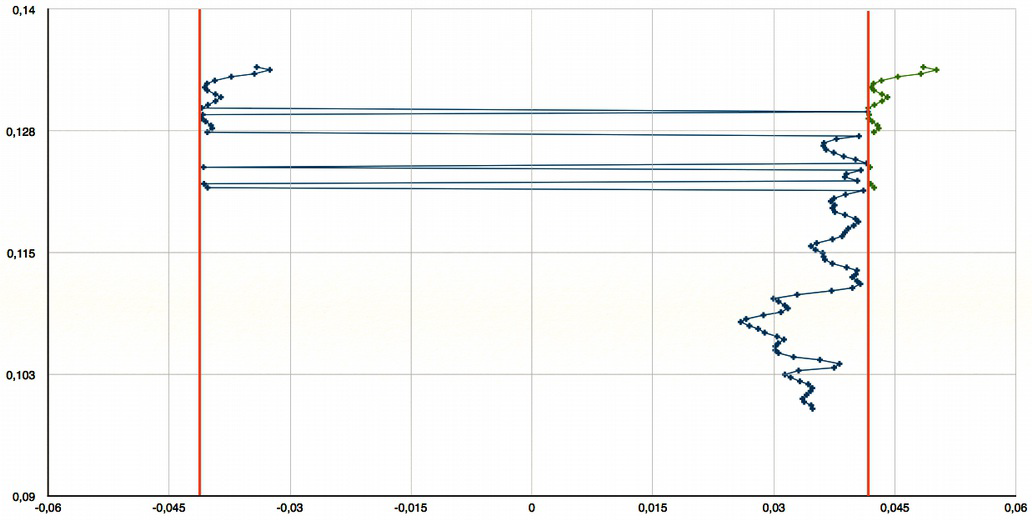
This phase jump results in a velocity jump that can be observed on a profile with a velocity gradient. The figure below shows the measurement on a profile with velocity increasing with the depth. The red lines show the velocity limits of the range; one can see that each velocity outside this range suffers from a jump that brings it inside the interval. Thus the instantaneous velocity (in green) is reduced in negative values when they overstep the highest limit of the range.

The velocity range for the projected velocities (as measured by the device) is given by:

$$R_{vp} = {{c⋅PRF} \over {2⋅f_0}}$$

with:

$PRF$: the Pulse Repetition Frequency [Hz],
$c$: the sound speed (about 1480m/s in water) [m/s],
$f_0$: the emission frequency [Hz].

Finally, it is the pulse repetition frequency (PRF) that will act on one side on the maximal exploration depth and on the other side on the maximal velocity. This limit is expressed by:

$$R_v⋅R_y = {{c^2⋅\tan{\beta}} \over {4⋅f_0}}$$

with:

$R_v$: the velocity range along the flow axis (equal to 2.6 m/s in the example above) [m/s].
$R_y$: the exploration depth (orthogonal to the main flow direction, the pipe diameter for example) [m].
$\beta$: the angle between the beam axis and the velocity vector.

The product of the velocity range and the exploration depth is thus fixed for a given setup.

The backscattered amplitude measurement is done simultaneously with the velocity measurement.

After each emitted pulse, the transducer receives the echoes from the particles crossing the acoustic beam. Thus the received acoustic wave corresponds to the sum of the echoes of each particle randomly distributed along the beam. This signal is thus stochastic.

For each cell, the device computes the voltage amplitude (RMS value, expressed in Volts) received by the transducer.

The usual shape of the amplitude profile is decreasing due to the diffusion of the ultrasounds by the particles in any direction and due to the wave attenuation by absorption. In order to compensate this decrease, the electronics controls the gain as a function of the depth. This gain is expressed as:

$$G_{dB}(r) = a_0 + a_1⋅r$$

with:

$G_{dB}$: the amplification gain in dB
$a_0$: the equivalent gain for a distance equal to zero (transducers surface),
$a_1$: the gain slope in dB/m,
$r$: the depth along the transducers axis.

The gain can be set in the range 20 to 68 dB for the UB-Lab and for the UB-Flow.

If the amplification gain is too high, there is a risk for the signal to saturate. If the gain is too low the signal-to-noise ratio may be bad.

The system presents a blind zone, just in front of the transducer, going from 2 to 20 mm depending on the transducer, the frequency and the concentration of particles. In this zone, the signal-to-noise ratio is low due to the ultrasonic emission: the transducer is blinded by the ultrasonic burst that has just been emitted.

Our devices are equipped with an automatic gain control algorithm that optimizes the gain over the full observed window with a logarithmic law. It is thus recommended to limit the number of cells to the area of interest so that the gain is well adapted to this area (and not influenced by the echoes after an interface for example).

Level measuring principle

The user can evaluate the water level (or of any other interface) by observing a strong variation of the backscattered amplitude gradient.

A script is available for this detection on our post-processing interface.

The usual shape of the amplitude profile is decreasing due to different factors:

The wave is attenuated by absorption due to viscous friction and relaxation, which depends on medium and sound frequency, and is described by:

$$I_{att}(z) = I_0⋅e^{- 2⋅α⋅z}$$

In water:
- $α = K f^2$
- $K = (2.4⋅10^{-3}⋅(T - 38)^2 + 1.5)⋅10^{-14}$
The ultrasound is scattered by the particles in any direction, also called diffusion. Crossing of medium interfaces also participates in diffusion through reflection and refraction.
The beam is diverging. See Tutorial What does the acoustic beam look like? How does it impact the measuring cell's geometry ?

The Doppler Signal-to-Noise Ratio (SNR) is given in dB. It gives information about the quality of the velocity estimation.

It is the ratio between the Doppler signal, which is coherent to the last emission, and the noise’s energy, so what remains in the signal and which is not coherent with this emission.

$$SNR_{Doppler} = 10⋅log({E_s \over E_n})$$

with:

$E_s$: the signal energy,
$E_n$: the noise energy

This is why we use the pulse coding, to make the echoes from the previous emissions non coherent and identifiable (see our FAQ on pulse coding).